|
|
|
Active Filter
Ronan ALLIBERT
Bsc Electrical and electronic engineering
Active filter design
Brian Temple
1/11/99
Active Filters design
Low pass filter with a cut off frequency of 2,5kHz
1st order active filter design
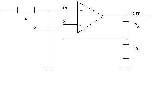
We need a gain of 2 so with the expression of the gain A=RA/RB+1 we see that RA should be equal to RB . Let say RA=RB =1k
WWe have now to choose R and calculate the value of C to get the right cut off frequency. Let say R=10k
Ww
c = 1/RC = 2 ? f = 2 ? x 2,5 x 103= 15708 rad.s-1
The denormalisation factor is 10k.
C = 1/(R x
w c)C = 1/(10 x 103 x 15708) = 6,3nF
Low pass 1st order active filter
fc=2,5kHz
RA=RB =1k
WR=10k
WC = 6,3nF
2nd order low pass active filter design

Sallen and key configuration
Butterworth response
Gain of 2/cut off frequency of 2,5 kHz
Parameters:
For a gain of two a normalised filter with a Butterworth response, has R1=R2=1
W C1"=0,874 and C2"=1,144.For a cut off frequency of 2,5kHz:
C1’=C1"/2
? fc and C2’=C2"/2? fcC1’=0,874/(2
? 2,5k)=5,56x10⁻⁵C2’= 1,144/(2
? 2,5k)=2,28x10⁻⁵Those values are given for R(=)= 1
W so we will now chose a value for R in order to get more practical values for C1 and C2.Let say R=1k
W so we get C1=C1’/R and C2=C2’/R.R=R1=R2=1k
WC1=55nF
C2=72nF
We have also to get values for RA and RB in order to get the next given equation true.
R1+R2
@ RARB/(RA+RB)RARB/(RA+RB)
@ 2k=> RA=RB=4k
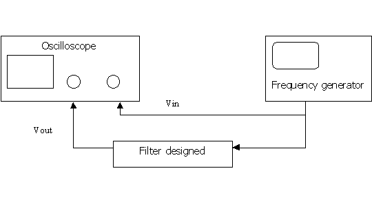
Next step of the work done was the measurements of the filter.
Protocol:
| Freq | 100 |
300 |
500 |
1000 |
1500 |
2000 |
2200 |
2400 |
2500 |
3000 |
3500 |
4000 |
5000 |
6000 |
10000 |
| Vin (mV) | 13 |
13 |
13 |
13 |
13 |
13 |
13 |
13 |
13 |
13 |
13 |
13 |
13 |
13 |
13 |
| Vout (mV) | 28 |
28 |
28 |
27 |
24 |
22 |
21 |
20 |
20 |
18 |
16 |
15 |
13 |
12 |
7 |
| Vin/Vout | 0,46 |
0,46 |
0,46 |
0,48 |
0,54 |
0,59 |
0,62 |
0,65 |
0,65 |
0,72 |
0,81 |
0,87 |
1 |
1,08 |
1,86 |
| -20log(Vin/Vout) | 6,74 |
6,74 |
6,74 |
6,38 |
5,35 |
4,58 |
4,15 |
3,74 |
3,74 |
2,85 |
1,83 |
1,21 |
0 |
-0,67 |
-5,39 |
Tab 1 : measurements of the first order low pass active filter with a cut off frequency of 2,5kHz
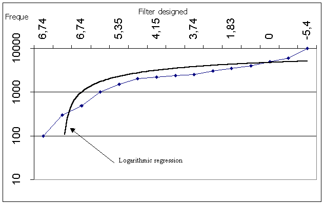
Graph 1 : Gain versus Frequency of the first order low pass active filter with a cut off frequency of 2,5kHz
We can see first that we have a gain of about two. Vout
@ 2Vin, at the beginning of the measurements.The cut off frequency is given for an attenuation of 3 dBs, in the tab 1 we can figure out that it is 2,4kHz, that is quite close to the wanted value. This difference can be explained by the different values of the components and their tolerance. We have a difference off 4%, and the tolerance is 5%.
| Freq | 100 |
500 |
1000 |
1500 |
1750 |
2000 |
2250 |
2500 |
2750 |
3000 |
3500 |
4000 |
5000 |
| Vin (mV) | 15 |
15 |
15 |
15 |
15 |
15 |
15 |
15 |
15 |
15 |
15 |
15 |
15 |
| Vout (mV) | 30 |
29 |
29 |
28 |
26 |
24 |
23 |
20 |
18 |
16 |
14 |
10 |
8 |
| Vin/Vout | 0 ,5 |
0,52 |
0,52 |
0,54 |
0,58 |
0,63 |
0,65 |
0,75 |
0,83 |
0,91 |
1,07 |
1,5 |
1,88 |
| -20log(Vin/Vout) | 6,02 |
5,68 |
5,68 |
5,35 |
4,73 |
4,01 |
3,74 |
2,5 |
1,62 |
0,82 |
-0,59 |
-3,5 |
-5,5 |
Tab 2 : measurements of the second order low pass active filter with a cut off frequency of 2,5kHz
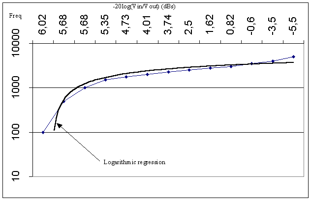
Graph 2 : Gain versus Frequency of the second order low pass active filter with a cut off frequency of 2,5kHz
We can see first that we have a gain of two. Vout = 2Vin, at the beginning of the measurements.
The cut off frequency is given for an attenuation of 3 dBs, in the tab 2 we can figure out that it is 2,25kHz and 2,5kHz, that is quite close to the wanted value. Again with a linear regression between this interval, we can see that at 3dBs (6,02-3 is about 3dBs), 2250+((2500-2250)X(3,74-3))/(3,74-2,5)
@ 2399Hz (the cut off frequency).This difference can be explained by the different values of the components and their tolerance. We have a difference off 4%, and the tolerance of the components is 5%.
Spiceage simulation Frequency response and coded circuit.
Y is the input of the whole filter, IN the + of the AOP, X the – of the AOP and OUT its output.
Low-pass filter response 1st order
* Low pass active filter with fc=2.5kHz and a gain of 2
* The library circuit is the OA741b.lib
*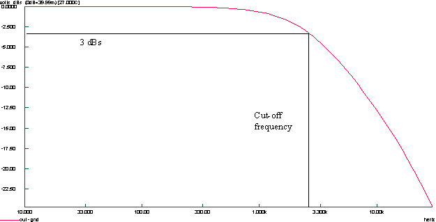
B 1 neg:gnd pos:Vcc+ v=15.00000
B 2 neg:gnd pos:Vcc- v=-15.0000
> OpAmp1 OA741b v-:Vcc- v+:Vcc+ out:out in-:X in+:in
V 1 -out:gnd +out:y v=20.0000m Ex=Sine Fr=6.00000k
R RA p1:out p2:X v=1.00000k %=5.00
R RB p1:X p2:gnd v=1.00000k %=5.00
C C1 p1:in p2:gnd v=6.37000n %=5.00
R R1 p1:in p2:y v=10.0000k %=5.00
We can’t figure out the gain with this software, but the cut off frequency is about 2,5kHz. The plotted simulation has been done with no tolerance, so this case is ideal. We have an attenuation of 20 dBs per decade.
Spiceage simulation for the second order filter
Again X is – for the AOP, OUT for its output, In for its + pin, Y is between R1 and R2 and Z is the input of the whole circuit.
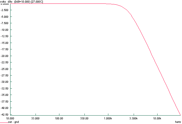 Low-pass filter response
second order
Low-pass filter response
second order
* Second order low pass active filter (butterworth) fc=2.5kHz and a gain of 2
* The library circuit is the OA1.lib
*
> oa1 oalin.lib in+:in in-:x out:out gnd:gnd
V 1 +out:z -out:gnd v=5.000000 Ex=Sine Fr=6.00000k
R RA p1:out p2:X v=4.00000k %=5.00
R RB p1:X p2:gnd v=4.00000k %=5.00
C C2 p1:in p2:gnd v=72.0000n %=5.00
R R2 p1:in p2:Y v=1.00000k %=5.00
C C1 p1:Y p2:out v=55.0000n %=5.00
R R1 p1:Y p2:Z v=1.00000k %=5.00
We can’t figure out the gain with this software, but the cut off frequency is about 2,5kHz. The plotted simulation has been done with no tolerance, so this case is ideal. We have an attenuation of 40 dBs per decade.
Results of both measurements and simulation were acceptable looking at the theoretical calculus done. The spiceage simulation for the second order filter was done with a different kind of AOP because the first gave wrong results for no apparent reason. The butterworth response has not been checked by the theoretic damping factor (unknown for a gain of two) but the general shape of the curve, shows the right response.